Latex-Template and information
The template for a bachelor or master thesis, or expose can be found here:
Please log in with your computer science account.
The LaTeX template is structured into a few folders and files:
parts: all text files for the chapters and sections and ..._acronyms.tex: the definitions of acronyms you use_bibliography.bib: the definitions of your BibTeX references_glossary.tex: the definitions of terminologies you use
template: all LaTeX style files for this template, that is ...custom_commands.sty: the definitions of custom commandscustom_listings.sty: definitions of languages for your listingstemplate.sty: the main file of this templatetitlepage_*.sty: the title page for the respective text type
data.sty: the document informationmain.tex: the main file of this document
Some of the files will be further explained in Structural elements.
You should also add some resource folders for images, tables, etc., depending on your needs.
Edit Helpers
This template provides four options that enable edit helpers: notes, coloredrefs, grid, and pagebreaks.
coloredrefs: colors all references and URLs blue. This is nice to keep in the digital version, but you might want to disable it before printing.
edit: enables the following four commands, which can help you to keep track of todos, notes, finished parts, and annotations from your reviewers.
\todo{message}to keep track of what you have to do (in red),\note{message}to make a simple note (in orange),\annot{Name}{message}to add an annotation by a reviewer (in orange),\done{}to simply mark something as done (in green).
grid: puts a grid behind the content and frames around the text. This can help to adjust and position figures, tables, and listings as well as to identify overlong lines.
pagebreaks: inserts a page break before every section, sub-section, and sub-sub-section. This shall just help to better navigate through the document but should not be used for the final, printed version.
Note that before finalizing this document you should deactivate the helpers. If you forgot to remove any todo, note, or annotation, you will be warned by a compiler error, whilst any remaining \done{} will be removed silently.
First Steps
- Fill in your information in
data.sty.
Last Steps
- Remove the edit helpers
edit,grid,pagebreaks. - You can keep
coloredrefsfor the digital version, but remove it for the printed one.
File Names
We encourage you to split your text into separate files. This way, you do not end up with one enormous file that contains your whole document. Use the command \input for inserting these files into the main.tex.
There are common ways of structuring these files, with pros and cons:
- Simple1: one file per chapter, e.g.,
introduction.tex - Simple2: one file per chapter and section (or even subsection), e.g.,
introduction.texandresearch_questions.tex - Prefix1: one file per chapter, files are prefixed by the chapter numbers, e.g.,
1_introduction.tex - Prefix2: one file per chapter and per section (or even subsection), prefixed by the chapter and section numbers, e.g.,
1_introduction.texand1_2_research_questions.tex - Nested1: one file and subdirectory per chapter, where the subdirectory contains one file per section, e.g.,
introduction.texandintroduction/research_questions.tex - Nested2: Nested1 with prefixes, e.g.,
1_introduction.texand1_introduction/2_research_questions.tex
These structures have pros and cons:
- Sorting: Overleaf sorts the files alphabetical by default (Simple1, Simple2, Nested1). Prefixing the files by the chapter (and section) numbers (Prefix1, Prefix2, and Nested2) sorts the files the same way as they appear in the text. However, if you need to add, move, or remove a section (or subsection), you need to adjust all subsequent file prefixes and update the
\inputcommands in yourmain.tex. Especially in the early phase, this can be a real waste of time. For Nested2, this problem is at least reduced. - File size: The files in Simple1 and Prefix1 are still large, and scrolling takes long. The other structures have smaller files, which eases scrolling.
- Searching: Overleaf does not provide a global search, just a file-wise one. You can search in the PDF using the browser's search and then jump to the respective source code, but only in compiled text and not in comments. Hence, searching is easier in Simple1 and Prefix1 if you need to search in comments.
Structural Elements
The template supports the following commands for structural elements:
\chapter{}\section{}\subsection{}\subsubsection{}\paragraph{}\subparagraph{}
Use the description environment for concise definitions or explanations.
In LaTeX, you initiate a new paragraph only with a blank line. This ensures proper text flow and indentation, especially at page breaks. Do not use \\ or \newline for starting new paragraphs; these commands do not create the correct paragraph structure. For additional vertical spacing, employ \vspace, \baselineskip, or alike.
Figures
Visual elements like images can significantly enhance the understanding of complex information at a glance. They add color and dynamics, offering a visual break from continuous, monotonous text, thus maintaining reader engagement. Therefore, do incorporate them effectively in your document to enrich the reader's experience and aid in the comprehension of your material.
Criteria for Figures
Your figures should adhere to specific criteria:
- Content: Select content that is most relevant and illustrative of your point.
- Resolution: Opt for scalable vector graphics (such as SVG) or high-resolution images (minimum 300dpi). For diagrams or charts, consider using LaTeX-native graphics like TikZ or PGF.
- Colors: The choice of color depends on your printing method:
- Colored: Use colors with significant contrast in hue, saturation, and lightness. You can find various color palettes online that suggest harmonious combinations. Ideally, choose palettes that are accessible to those with color vision deficiencies [1] [2]. In your descriptions, opt for universally recognized color names like "dark red" or "light blue" rather than obscure ones.
- Gray scale: If printing in gray scale, ensure adequate contrast between different shades. Avoid using very light grays as they might not print well. In diagrams, differentiate elements through distinct shapes or strokes, as you would with color.
- Dimensions: Figures do not necessarily have to span the entire page width. They should be appropriately scaled (e.g., to 60%) and centered.
- Scaling: Maintain consistent scale across similar types of figures, such as bar charts, ensuring uniform bar widths and font sizes.
- Labeling: Ensure that all diagrams are fully labeled, particularly the axes. Utilize legends or detailed captions to explain each component's significance. Captions appear in the lists of figures and should be informative yet concise; if needed, provide a shortened version for lengthy descriptions.
Layout
LaTeX's layout algorithms automatically place figures, tables, and listings in your text.
Unfortunately, these positions are not always ideal. Still, you should not waste time tweaking their positions throughout the writing process; it's more efficient to adjust their placement only towards the end, once your full text is finished.
If you need to reposition these elements manually, it is advisable to position them preferably only at the top or only at the bottom of the page. This approach prevents isolated lines of text from getting sandwiched between them.
When multiple graphics are related or shall be compared, you can place them together on a special page. This page will then contain only graphics, no text.
In the figure, table, and listings environments, prefer the position arguments t for top of the page, or p for a special page.
Simple Figures
If you have an existing image, including it in your document is straightforward, as demonstrated with Figure 1. Additionally, it's essential to accompany each image with a descriptive caption that explains the image's content, including relevant details like colors, shapes, and groups. This is also the appropriate place to cite the source of the image using the \cite command if it is not originally yours. For the List of Figures, you may provide a shortened version of the caption if necessary. Lastly, assigning a label to the figure is crucial, as it enables you to refer to the figure elsewhere in your text efficiently. This approach ensures that your figures are not only well-integrated but also informative and correctly referenced.

\begin{figure}[t]
  \centering
  \includegraphics[width=.3\textwidth]{imgs/latex}
  \caption[Example figure]{An included image file showing the writing \LaTeX{}. Source: \cite{sample:wiki:latexlogo}}
  \label{fig:sample-latex}
\end{figure}
Subfigures
If you provide related figures, use subfigures as shown in Figure 2. Assign individual captions and labels to each subfigure and an overall caption and label for the entire group.

\begin{figure}[t]
  \centering
  \subcaptionbox
    [Black text on white background]
    {Black text on white background. Source: [1]}
    [.48\textwidth]
    {\includegraphics{samples/imgs/latex}}
  \hfill
  \subcaptionbox
    [White text on black background]
    {White text on black background. Adopted from: [1]}
    [.48\textwidth]
    {\includegraphics{samples/imgs/latex_dark}}
  \caption[Figure with two subfigures]
          {An example figure that contains two related subfigures.}
  \label{fig:subfigures}
\end{figure}
TikZ and PGF
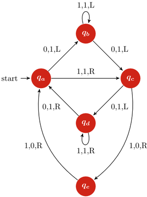
For creating graphs like those in Figures 3 and 4, consider using the TikZ and PGF packages. With these, similar to LaTeX, you simply supply the content and select a style; the layout is then generated automatically.
Many mathematics and statistics applications support direct export to TikZ and PGF formats. In R, you can use the tikzDevice library, and in Python projects with matplotlib, you can use the tikzplotlib library to transform your graph into TikZ.
Note, TikZ consists of various libraries tailored for specific functionalities, so you may need to incorporate additional ones depending on your needs. To do this, include the necessary libraries using the command \usetikzlibrary in your main.tex file.
\begin{tikzpicture}[->,>=stealth',shorten >=1pt,auto,
    node distance=2.8cm,semithick]
  \tikzstyle{every state}=[fill=myred,draw=none,text=white,font=\boldmath]
  \node[initial,state] (A)                    {$q_a$};
  \node[state]         (B) [above right of=A] {$q_b$};
  \node[state]         (D) [below right of=A] {$q_d$};
  \node[state]         (C) [below right of=B] {$q_c$};
  \node[state]         (E) [below of=D]       {$q_e$};
  \path (A) edge              node {0,1,L} (B)
            edge              node {1,1,R} (C)
        (B) edge [loop above] node {1,1,L} (B)
            edge              node {0,1,L} (C)
        (C) edge              node {0,1,L} (D)
            edge [bend left]  node {1,0,R} (E)
        (D) edge [loop below] node {1,1,R} (D)
            edge              node {0,1,R} (A)
        (E) edge [bend left]  node {1,0,R} (A);
\end{tikzpicture}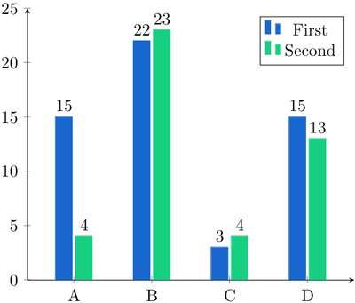
\begin{tikzpicture}
  \begin{axis}[
      ybar,
      axis x line = bottom,
      axis y line = left,
      ytick pos = left,
      enlarge x limits  = 0.2,
      symbolic x coords = {A, B, C, D},
      nodes near coords,
      ymin = 0,
      ymax = 25,
      legend pos=north east
  ]
  \addplot[fill=myblue, draw=myblue] coordinates {
      (A, 15)
      (B, 22)
      (C, 3)
      (D, 15)
  };
  \addplot[fill=mygreen, draw=mygreen] coordinates {
      (A, 4)
      (B, 23)
      (C, 4)
      (D, 13)
  };
  \legend{First, Second}
  \end{axis}
\end{tikzpicture}Tables
Utilize tables to present structured data effectively, like comparisons or evaluation results.
Ensure all essential information is included and clearly label each column and/or row. Also, provide a descriptive caption to concisely explain the table's content.
However, avoid overcrowding tables. It's often more effective to split dense tables into smaller ones to enhance clarity and underscore their significance.
In terms of design, use lines sparingly as separators: typically, a table requires only three lines:
\topruleabove the header,\midrulebelow the header, and\bottomruleat the bottom.
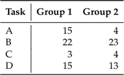
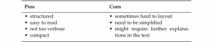
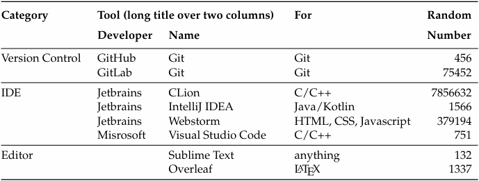
This minimalist approach takes advantage of cell alignment and spacing to naturally delineate the data. For more complex structures, like in Table 2, only a few additional lines may be necessary.
Creating Tables
Creating tables manually is a very tedious task. We recommend the Tables Generator that provides you with a graphical user interface.
Table Environments
LaTeX offers several table environments, including tabular, tabular*, and tabularx. These differ in layout, column styling, and compatibility. Choose the format that best fits your data. While tabular* is a good starting point, switch to tabular or tabularx as needed based on the specific requirements of your table. For instance, use tabular* for Table 2 and opt for tabular or tabularx if the table includes lists or more complex data arrangements, similar to Table 1.
\begin{table}[]
    \centering
    \begin{tabular}{l|rr}
        \toprule
        \thead{Task} & \thead{Group 1} & \thead{Group 2} \\ \midrule
        A            & 15              &  4              \\
        B            & 22              & 23              \\
        C            &  3              &  4              \\
        D            & 15              & 13              \\ \bottomrule
    \end{tabular}
    \caption{A simple table (tabular)}
    \label{tab:simple}
\end{table}
\RequirePackage{tabularx} // from template.sty
  \begin{table}[t]
    \centering
    \begin{tabularx}{0.8\linewidth}{XX}                    \toprule
      \thead{Pros} & \thead{Cons}                       \\ \midrule
      \vspace{-\topsep}
      \begin{itemize}[topsep=0pt, partopsep=0pt, nosep, before=\setstretch{1}]
        \item structured
        \item easy to read
        \item not too verbose
        \item compact
      \end{itemize}
      \vspace{-\topsep}
      &
      \vspace{-\topsep}
      \begin{itemize}[topsep=0pt, partopsep=0pt, nosep, before=\setstretch{1}]
        \item sometimes hard to layout
        \item need to be simplified
        \item might require further explanations in the text
      \end{itemize}
      \vspace{-\topsep}                                 \\[-\topsep] \bottomrule
    \end{tabularx}
    \caption{A table with enumerations (tabularx)}
    \label{table:sample-pros-cons}
  \end{table}
\RequirePackage{multicol} // from template.sty
  \begin{table}[t]
    \centering
	\begin{tabular*}{\linewidth}{@{\extracolsep{\fill}}llllr}                                                          \toprule
	\thead{Category}
            & \multicolumn{2}{l}{\thead{Tool (long title over two columns)}}
                                             & \thead{For}           & \thead[l]{Random} \\
	        & \thead{Developer} & thead{Name} &                      & \thead[l]{Number} \\ \midrule
	Version & GitHub    & Git                & Git                   & 456               \\
	Control & GitLab    & Git                & Git                   & 75452             \\ \midrule
	IDE     & Jetbrains & CLion              & C/C++                 & 7856632           \\
	        & Jetbrains & IntelliJ IDEA      & Java/Kotlin           & 1566              \\
	        & Jetbrains & Webstorm           & HTML, CSS, Javascript & 379194            \\
	        & Misrosoft & Visual Studio Code & C/C++                 & 751               \\ \midrule
	Editor  &           & Sublime Text       & anything              & 132               \\
	        &           & Overleaf           & \LaTeX{}              & 1337              \\ \bottomrule
	\end{tabular*}
	\caption{A complex table (tabular*)}
	\label{table:sample-tools}
  \end{table}
Listings
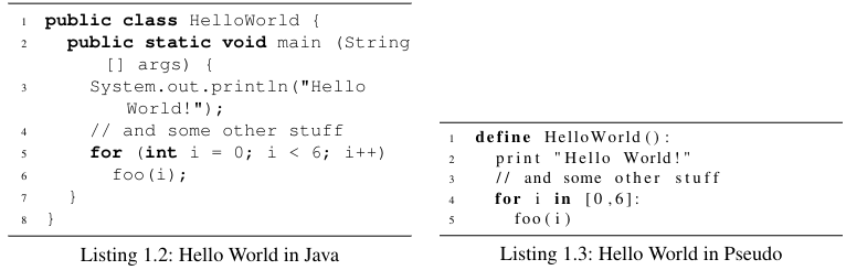
When you're explaining an algorithm or a complex workflow, using source code or pseudocode can be exceptionally effective. LaTeX offers the listings environment, which accommodates syntax highlighting for various programming languages, as well as for custom-defined and -styled languages. For instance, Listing 1 showcases a "Hello World" example in Java, while Listing 3 presents the equivalent in pseudocode. Notably, "Pseudo" is a custom language defined in template/custom_listings.sty.
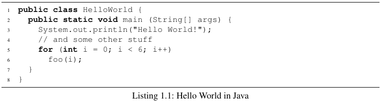
\begin{listingsbox}[t]
  \lstinputlisting[
    language=Java,
    label=lst:sample-java,
    caption={Hello World in Java}
  ]{listings/HelloWorld.java}
\end{listingsbox}
Listings Side by Side
The listingsbox environment automatically manages the spacing around your code block. If you need to display two listings adjacent to each other, utilize the sublistingsbox environment. Unlike figures and subfigures, when using sublistingsboxes, you do not need to provide separate captions and labels for each listingsbox.
\begin{listingsbox}[t]
    \begin{sublistingsbox}
        \lstinputlisting[
            language=Java,
            label=lst:sample-java,
            caption={Hello World in Java}
        ]{listings/HelloWorld.java}
    \end{sublistingsbox}
    \hfill
    \begin{sublistingsbox}
        \lstinputlisting[
            language=pseudo,
            label=lst:sample-pseudo,
            caption={Hello World in Pseudo}
        ]{listings/HelloWorld.pseudo}
    \end{sublistingsbox}
\end{listingsbox}
Labels
You should discuss the code within your text, even if the code appears self-explanatory. Make use of labels to refer to specific code lines. For example:
Line 3 in Listing 1 and line 2 in Listing 2 highlight critical sections of the code.
To achieve this, enclose the \label command within the language-specific escape characters (e.g., $|$ for Java and § for Pseudo).
public class HelloWorld {
  public static void main (String[] args) {
    System.out.println("Hello World!"); |\label{line:sample-java-print}|
    // and some other stuff
    for (int i = 0; i < 6; i++)
      foo(i);
  }
}
define HelloWorld():
  print "Hello World!"    §\label{line:sample-pseudo-print}§
  // and some other stuff
  for i in [0,6]:
    foo(i)
Citations
Relevant Commands
Cite a source by referencing the label of a BibTeX entry (see next section):
We base our evaluation on that from \cite{author2023}.
Use the correct quotation marks. Do not just use the single or double quotes from your keyboard. Instead:
``Text'' \enquote{Text} `Text' \enquote*{Text}
For longer quotes, you can optionally use the quote environment (provided by our template):
\begin{quote}[Whitten et al. \cite{sample:whitten1999johnny}] ``It is well known that the security of a networked computer is only as strong as its weakest component.''
\end{quote}
BibTeX
BibTeX formats your bibliography automatically at the end of your text; you just need to provide the relevant information in BibTeX entries. Many science-related websites, including conference sites, Google Scholar, and Wikipedia, supply these BibTeX entries. However, the level of detail and their values may vary across sites, hence requiring some cleanup on your part.
Below are the most crucial source types you will need and their expected formatting1.
Some General Rules:
- Please ensure these details are included and remove any additional information. If a digital object identifier (DOI) is available, you can keep it.
- Using quotation marks or braces around the values makes no difference.
- For titles featuring subtitles, divide them using a colon, dash, or period.
- Regarding author names, adhere to the syntax
{Doe, John}. For collaborations involving two or more authors, link them with "and":{Doe, Joe and Smith, Jane}. - To prevent the misinterpretation of company names or similar entities as individual names, enclose them in additional braces:
{{Super Important Company} and Doe, John}or"{Super Important Company} and Doe, John". - The BibTeX entries are identified by a label, such as "author2023" or "website2023" in the examples below. You can select any unique name that suits you; opt for those that you can most easily recognize and remember.
- If information is missing, write "unknown". For websites, if no author is explicitly mentioned, use the website owner, which can be found in the Impressum. For Git repositories and similar platforms, use the repository owner as the author.
Conference/workshop/... paper:
@inproceedings{author2023,
    title        = {An Analysis of Example},
    author       = {John Smith and Jane Doe},
    year         = {2023},
    booktitle    = {Proceedings of the International Conference on Example},
    publisher    = {ACM Press},
    volume       = {1},
    number       = {2},
    pages        = {123--130}

}
Article:
@article{author2023, author = {Jane Smith},
title = {Title of the Article},
journal = {Name of the Journal},
year = {2023},
volume = {4},
number = {2},
pages = {100-105}
}
Book:
@book{author2023,
    author    = {Jane Smith},
    title     = {Title of the Book},
    publisher = {Publishing House},
    year      = {2023},
    address   = {City of Publication},
    edition   = {3rd}
}
Website:
@misc{website2023,
    author    = {John Doe},
    title     = {Title of the Web Page},
    year      = {2023},
    url       = {http://www.example.com},
    note      = {Accessed on: 2023-10-04}
}
Personal conversation or interview:
@misc{website2023,
    author    = {John Doe},
    title     = {Personal conversation with the developer of SomeAwesomeTool},
    note      = {2023-10-04}
}
1. Examples adopted from: https://bibtex.eu/
Acronyms
For long terminologies, you might want to use acronyms, such as "SSL" for "Secure Sockets Layer". Introduce each acronym at its first occurrence in your document, and subsequently, refer to the acronym alone. However, this rule does not apply to headings; headings should generally not contain acronyms unless they have been previously introduced and are well-understood by the intended reader.
The Hypertext Transfer Protocol Secure (HTTPS) extends the Hypertext Transfer Protocol (HTTP) with Transport Layer Security (TLS), where TLS is a successor of Secure Sockets Layer (SSL).
In LaTeX, the commands \acrshort, \acrlong, and \acrfull ensure accurate acronym usage, preventing misdefinition or misspelling. For example:
The \acrfull{https} extends the \acrfull{http} with \acrfull{tls},
where \acrshort{tls} is a successor of \acrfull{ssl}.
Furthermore, compile an overview of the utilized acronyms to append after the table of contents. Place these definitions in the parts/_acronyms.tex file. Example:
\newacronym{http}{HTTP}{Hypertext Transfer Protocol}

\newacronym{https}{HTTPS}{Hypertext Transfer Protocol Secure}

\newacronym{ssl}{SSL}{Secure Sockets Layer}

\newacronym{tls}{TLS}{Transport Layer Security}
Glossary
The glossary lists all the terms used throughout your document. You should define these terms in the parts/_glossary.tex file, each with a brief description. For example:
Glossary: An alphabetical list of terms accompanied by brief explanations.
Thesis: Scholarly documents detailing research and findings, required for academic degrees.
\newglossaryentry{glossary}{

    name=glossary,
    plural=glossaries,

    description={An alphabetic list of terms with brief descriptions.}

}

\newglossaryentry{thesis}{
    name=thesis,
    plural=theses,
    description={Scholarly document detailing research and findings, required for academic degrees.}

}
To use these glossary entries within your text, use the \gls{} command.